File:Effect of circular convolution on discrete Hilbert transform.png
Jump to navigation
Jump to search

Size of this preview: 800 × 421 pixels. Other resolutions: 320 × 168 pixels | 640 × 337 pixels | 1,156 × 608 pixels.
Original file (1,156 × 608 pixels, file size: 100 KB, MIME type: image/png)
Summary
| Description |
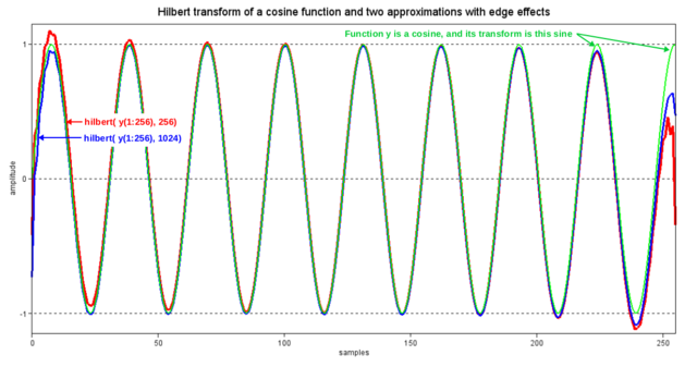
English: The Hilbert transform of cos(ωt) is sin(ωt). When a finite segment of cos(ωt) is transformed, edge effects inevitably occur. Using a segment length of 256 samples, this figure shows a sine function and two approximate Hilbert transforms computed by the MATLAB library function, hilbert(·), which supports optional zero-filling of the segment to be transformed. The red graph is the result of no zero-filling, and the blue graph is the result of 300% zero-filling. In the latter case, the edge effects are almost all due to the rise and fall times of the Hilbert transform's 2/(πn) impulse response. In the "red" case, we have the added effect of circular convolution. In other words, in the blue case, distortion occurs when some of the filter taps are coinciding with zeros, instead of with samples of cos(ωt). And in the red case, those same taps are coinciding with wrapped-around (and out-of-phase) samples of cos(ωt). |
|||
| Date | ||||
| Source | Own work | |||
| Author | Bob K | |||
| Permission (Reusing this file) |
I, the copyright holder of this work, hereby publish it under the following license:
|
|||
| PNG development | This PNG graphic was created with LibreOffice. |
|||
| Source file | Scilab codeN=256;
x=0:N-1;
cycles_per_segment = 8.2888; // empirical value that displays edge effects well
cycles_per_sample = cycles_per_segment/N;
Yreal = cos(2*%pi*cycles_per_sample*x); // function to be transformed
Ans = sin(2*%pi*cycles_per_sample*x); // the ideal answer
H1 = imag(hilbert(Yreal)); // no zero-filling
H2 = imag(hilbert([Yreal zeros(1,1024-N)])); // zero-filling
// Display the results
red=5; blue=2; green=3; black=1; // based on a call to getcolor()
top=green; middle=blue; bottom=red;
plot2d(x', [H1' H2(1:N)' Ans'], style=[bottom middle top], rect=[0,-1.15,N-1,1.15]);
a = gca();
a.box = "on";
a.font_size=2; //set the tics label font size
a.visible = "on";
a.grid = [-1,0];
a.auto_ticks = ["off","off","off"]
a.y_ticks = tlist(["ticks", "locations", "labels"], [-1 0 1], ["-1" "0" "1"]);
a.x_ticks = tlist(["ticks", "locations", "labels"], [0 50 100 150 200 250], ["0" "50" "100" "150" "200" "250"]);
//a.children.children.thickness=2; // set line thickness of plots
top=1; middle=2; bottom=3;
a.children.children(top).thickness=2;
a.children.children(middle).thickness=3;
a.children.children(bottom).thickness=4;
xlabel("samples", "fontsize", 2)
ylabel("amplitude", "fontsize", 2)
title("Hilbert transform of a cosine function and two approximations with edge effects", "fontsize", 4)
|
See also
File history
Click on a date/time to view the file as it appeared at that time.
| Date/Time | Thumbnail | Dimensions | User | Comment | |
|---|---|---|---|---|---|
| current | 12:58, 9 February 2016 | | 1,156 × 608 (100 KB) | wikimediacommons>Bob K | Show the sine function and 2 approximations, instead of the 2 difference functions. |
File usage
There are no pages that use this file.