File:Hamiltonian flow classical.gif
From formulasearchengine
Jump to navigation
Jump to search
Hamiltonian_flow_classical.gif (195 × 390 pixels, file size: 172 KB, MIME type: image/gif, looped, 86 frames, 26 s)
This file is from Wikimedia Commons and may be used by other projects. The description on its file description page there is shown below.
Summary
| DescriptionHamiltonian flow classical.gif |
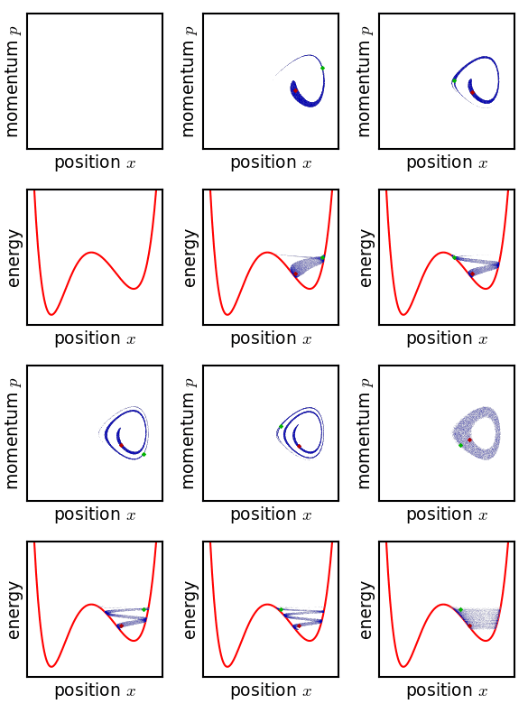
English: Flow of a statistical ensemble in the potential x**6 + 4*x**3 - 5*x**2 - 4*x. Over long times it becomes swirled up, and appears to become a smooth and stable distribution. However, this stability is an artifact of the pixelization (the actual structure is too fine to perceive). This animation is inspired by a discussion of Gibbs in his 1902 wikisource:Elementary Principles in Statistical Mechanics, Chapter XII, p. 143: "Tendency in an ensemble of isolated systems toward a state of statistical equilibrium". A quantum version of this can be found at File:Hamiltonian flow quantum.webm |
| Date | |
| Source | Own work |
| Author | Nanite |
Source
This plot was created with Matplotlib.
This image was created with ImageMagick.
Python source code. Requires matplotlib ImageMagick. Possibly does not run in Windows.
from pylab import *
import subprocess
import sys
import os

figformat = '.png'
seterr(divide='ignore')
rcParams['font.size'] = 9

#define color map that is transparent for low values, and dark blue for high values.
# weighted to show low probabilities well
cdic = {'red':   [(0,0,0),(1,0,0)],
        'green': [(0,0,0),(1,0,0)],
        'blue':  [(0,0.7,0.7),(1,0.7,0.7)],
        'alpha': [(0,0,0),
                  (0.1,0.4,0.4),
                  (0.2,0.6,0.6),
                  (0.4,0.8,0.8),
                  (0.6,0.9,0.9),
                  (1,1,1)]}
cm_prob = matplotlib.colors.LinearSegmentedColormap('prob',cdic,N=640)

### System dynamics ###

# potential is a polynomial
potential_coefs = array([1,0,0,4,-5,-4,0],'d')
def potential(x,t):
    return polyval(potential_coefs,x)

# force function is its derivative.
force_coefs = (potential_coefs*arange(len(potential_coefs)-1,-1,-1))[:-1]
def force(x,t):
    """ derivative of potential(x) """
    return polyval(force_coefs,x)
invmass = 1.0
dt = 0.03

def motion(t,x,p):
    """ returns dx/dt, dp/dt """
    return p*invmass, -force(x,t)

cur_x = -0.1
cur_p = 0

def rkky_step(t, x_i, p_i, dt):
    kx1,kp1 = motion(t, x_i, p_i)
    dt2 = 0.5*dt
    kx2,kp2 = motion(t+dt2, x_i+dt2*kx1, p_i+dt2*kp1)
    kx3,kp3 = motion(t+dt2, x_i+dt2*kx2, p_i+dt2*kp2)
    kx4,kp4 = motion(t+dt, x_i+dt*kx3, p_i+dt*kp3)
    newx = x_i + (dt/6.0)*(kx1 + 2.0*kx2 + 2.0*kx3 + kx4)
    newp = p_i + (dt/6.0)*(kp1 + 2.0*kp2 + 2.0*kp3 + kp4)
    return newx, newp

### Setup ensemble points ###

# most are randomly chosen
x = 0 + 0.5*rand(20000)
p = -1.0 + 2.0*rand(20000)

# the pilot points are set manually
x[0] = 0;    p[0] = 0
x[1] = 0.4;  p[1] = 0.0
pilots = [0,1]
pilot_colors = {
       0: (0,0.7,0),
       1: (0.7,0,0)}
E = potential(x,0) + 0.5*invmass*p**2

### set up plot limits and histogram bins ###
xedges = linspace(-2.1,1.7,151)
pedges = linspace(-7.5,7.5,151)
Eedges = linspace(-9,9,151)
pix = 150
extent = [xedges[0], xedges[-1], pedges[-1], pedges[0]]
H = histogram2d(x,p,bins=[xedges,pedges])[0].transpose()
cmax = amax(H)*0.8

extenten = [xedges[0], xedges[-1], Eedges[-1], Eedges[0]]
Hen = histogram2d(x,E,bins=[xedges,Eedges])[0].transpose()
cmaxen = amax(Hen)*0.3

fig = figure(1)
ysize = 2.6
xsize = 1.3
fig.set_size_inches(xsize,ysize)

### Prepare lower plot ###
axen = axes((0.2/xsize,0.2/ysize,1.0/xsize,1.0/ysize),frameon=True)
axen.xaxis.set_ticks([])
axen.xaxis.labelpad = 2
axen.yaxis.set_ticks([])
axen.yaxis.labelpad = 2
xlim(-2.1,1.7)
ylim(-9,9)
xlabel('position $x$')
ylabel('energy')
potx = linspace(-2.1,1.7,151)

### Prepare upper plot ###
ax = axes((0.2/xsize,1.5/ysize,1.0/xsize,1.0/ysize),frameon=True)
ax.xaxis.set_ticks([])
ax.xaxis.labelpad = 2
ax.yaxis.set_ticks([])
ax.yaxis.labelpad = 2
xlim(-2.1,1.7)
ylim(-7.5,7.5)
xlabel('position $x$')
ylabel('momentum $p$')

### Start running simulation ###
frames = list()
delays = list()
framemod = 5
frame = "frames/background"+figformat
savefig(frame,dpi=pix)
frames.append(frame)
delays.append(16)

print "generating frames...  0%",
sys.stdout.flush()
savesteps = range(0,401,framemod) + [600, 1000, 2000, 6000]
delays += [10]*len(savesteps)
delays[1] = 200
delays[-5:] = [100,200,200,200,400]
totalsteps = max(savesteps)+1
for step in range(totalsteps):
    if step % 20 == 0:
        print "\b\b\b\b\b{0:3}%".format(int(round(step*100.0/totalsteps))),
        sys.stdout.flush()
    if step in savesteps:
        # Every several frames, do a plot
        remlist = list()

        sca(ax)
        H = histogram2d(x,p,bins=[xedges,pedges])[0].transpose()
        remlist.append(imshow(H, extent=extent, cmap=cm_prob, interpolation='none', aspect='auto'))
        remlist[-1].set_clim(0,cmax)
        for i in pilots:
            remlist += plot(x[i], p[i], '.', color=pilot_colors[i], markersize=3)

        E = potential(x,step*dt) + 0.5*invmass*p**2
        sca(axen)
        pot = potential(potx,step*dt)
        remlist += plot(potx,pot,color='r',zorder=0)
        Hen = histogram2d(x,E,bins=[xedges,Eedges])[0].transpose()
        remlist.append(imshow(Hen, extent=extenten, cmap=cm_prob, interpolation='none', aspect='auto',zorder=1))
        remlist[-1].set_clim(0,cmaxen)
        for i in pilots:
            remlist += plot(x[i], E[i], '.', color=pilot_colors[i], markersize=3)

        frame = "frames/frame"+str(step)+figformat
        savefig(frame,dpi=pix)
        frames.append(frame)
        # Clear out updated stuff.
        for r in remlist: r.remove()
    x, p = rkky_step(step*dt, x, p,dt)
print "\b\b\b\b\b      done"

assert(len(delays) == len(frames))

### Assemble animation using ImageMagick ###
calllist = 'convert -dispose Background'.split()
for delay,frame in zip(delays,frames):
    calllist += ['-delay',str(delay)]
    calllist += [frame]
calllist += '-loop 0 -layers Optimize _animation.gif'.split()
f = open('anim_command.txt','w')
f.write(' '.join(calllist)+'\n')
f.close()

print "composing into animated gif...",
sys.stdout.flush()
subprocess.call(calllist)
print "      done"
os.rename('_animation.gif','animation.gif')
Licensing
I, the copyright holder of this work, hereby publish it under the following license:
| This file is made available under the Creative Commons CC0 1.0 Universal Public Domain Dedication. | |
| The person who associated a work with this deed has dedicated the work to the public domain by waiving all of their rights to the work worldwide under copyright law, including all related and neighboring rights, to the extent allowed by law. You can copy, modify, distribute and perform the work, even for commercial purposes, all without asking permission.
http://creativecommons.org/publicdomain/zero/1.0/deed.enCC0Creative Commons Zero, Public Domain Dedicationfalsefalse |
Captions
Add a one-line explanation of what this file represents
Items portrayed in this file
depicts
27 October 2013
image/gif
File history
Click on a date/time to view the file as it appeared at that time.
| Date/Time | Thumbnail | Dimensions | User | Comment | |
|---|---|---|---|---|---|
| current | 10:57, 27 October 2013 |  | 195 × 390 (172 KB) | wikimediacommons>Nanite | Added potential plot (with bonus ensemble histogram in E,x), as well as a couple of "pilot" systems. |
File usage
There are no pages that use this file.
