File:Heteroclinic orbit in pendulum phaseportrait.png
Jump to navigation
Jump to search

Size of this preview: 800 × 416 pixels. Other resolutions: 320 × 166 pixels | 640 × 333 pixels | 1,017 × 529 pixels.
Original file (1,017 × 529 pixels, file size: 15 KB, MIME type: image/png)
Summary
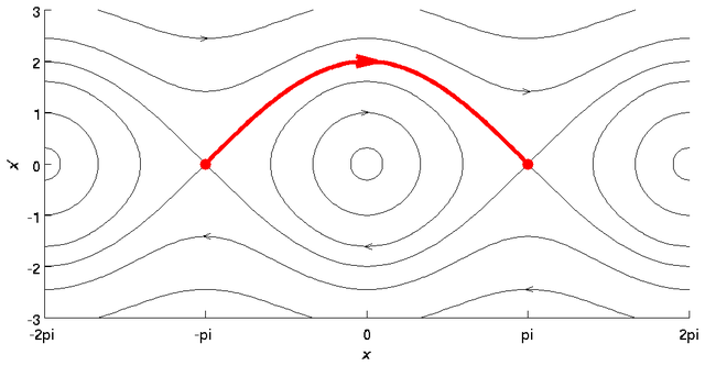
| Description | Phaseportrait for the pendulum equation with the heteroclinic orbit highlighted. Created by Jitse Niesen using Matlab. |
| Date | 29 June 2006 (original upload date) |
| Source | No machine-readable source provided. Own work assumed (based on copyright claims). |
| Author | No machine-readable author provided. Jitse Niesen assumed (based on copyright claims). |
Discussion
How come the orbit isn't called homoclinic? The domain is periodic: starting and ending point are the same.
- That depends on what you consider as the domain. If the domain is a circle (and hence periodic), which is the most natural choice, then you're right and the orbit is homoclinic. If the domain is R, the set of real numbers, then the starting and ending point are not the same. But you certainly have a point that this is a confusing example; thanks for that. -- Jitse Niesen 06:45, 2 February 2007 (UTC)
Licensing
| I, the copyright holder of this work, release this work into the public domain. This applies worldwide. In some countries this may not be legally possible; if so: I grant anyone the right to use this work for any purpose, without any conditions, unless such conditions are required by law. |
Matlab source
clf;
axis([-2*pi 2*pi -3 3]);
daspect([1 1 1]);
hold on;

% Draw constant energy contours
qs = linspace(-2*pi, 2*pi, 101);
[Q,P] = meshgrid(qs, linspace(-3,3));
H = P.*P/2 - cos(Q);
contour(Q,P,H, [-0.95 -0.5 0.3  2 4], 'k');

% Draw energy = 0 contour
ps = sqrt(2+2*cos(qs));
plot(qs,ps, 'k');
plot(qs,-ps, 'k');

% Draw heteroclinic connection
qs = linspace(-pi, pi, 101);
ps = sqrt(2+2*cos(qs));
plot(qs,ps, 'r', 'LineWidth', 3);
plot([-pi pi], [0 0], 'r.', 'MarkerSize', 25);

% Arrows
plot(-pi+[-0.10 0.05], sqrt(6)+[0.05 0], 'k');
plot(-pi+[-0.10 0.05], sqrt(6)+[-0.05 0], 'k');
plot(pi+[-0.10 0.05], sqrt(2)+[0.05 0], 'k');
plot(pi+[-0.10 0.05], sqrt(2)+[-0.05 0], 'k');
plot([-0.10 0.05], [1.05 1], 'k');
plot([-0.10 0.05], [0.95 1], 'k');
plot([0.10 -0.05], -sqrt(2.6)+[0.05 0], 'k');
plot([0.10 -0.05], -sqrt(2.6)+[-0.05 0], 'k');
plot(-pi+[0.10 -0.05], -sqrt(2)+[0.05 0], 'k');
plot(-pi+[0.10 -0.05], -sqrt(2)+[-0.05 0], 'k');
plot(pi+[0.10 -0.05], -sqrt(6)+[0.05 0], 'k');
plot(pi+[0.10 -0.05], -sqrt(6)+[-0.05 0], 'k');
plot([-0.2 0.2], [2.1 2], 'r', 'LineWidth', 3);
plot([-0.2 0.2], [1.9 2], 'r', 'LineWidth', 3);

% Axes
xlabel('\it{x}');
ylabel('\it{x}''');
set(gca, 'XTick', [-2*pi -pi 0 pi 2*pi]);
set(gca, 'XTickLabel', {'-2pi' '-pi' '0' 'pi' '2pi'});

% Print
print -dpng 'heteroclinic_tmp.png';
system('convert -trim -bordercolor white -border 10 +repage heteroclinic_tmp.png heteroclinic.png');
File history
Click on a date/time to view the file as it appeared at that time.
| Date/Time | Thumbnail | Dimensions | User | Comment | |
|---|---|---|---|---|---|
| current | 12:50, 29 June 2006 | | 1,017 × 529 (15 KB) | wikimediacommons>Jitse Niesen | Phaseportrait for the pendulum equation with the heteroclinic orbit highlighted. Created by ~~~ using Matlab. |
File usage
There are no pages that use this file.